Room no. 308
The room of our random experiments
Gradient Evolution
by 308
Evolution has always seemed to us a very fascinating theory - random genetic mutations leading to all sorts of weird creations, specialized for different tasks. In other words, it leads to optimizations on very complex, natural functions. Evolution makes sure that the species that fit their natural environment survive, while others perish.
Naturally, this has led to many attempts to replicate this procedure in more controlled settings. A whole class of algorithms called Evolutionary algorithms have been discovered (invented? this is a deeper question for another time) that are inspired from natural evolution. Here we discuss one such algorithm that we stumbled upon.
Optimization and Neural Nets
Nowadays, neural networks are used to model a large class of problems. Consider the problem of an AI playing some game. We want to “learn” a neural network such that, given the input parameter vector, it outputs the action (the input might be anything from a few numbers representing some state of the game, or the entire RAM at some stage of the game).
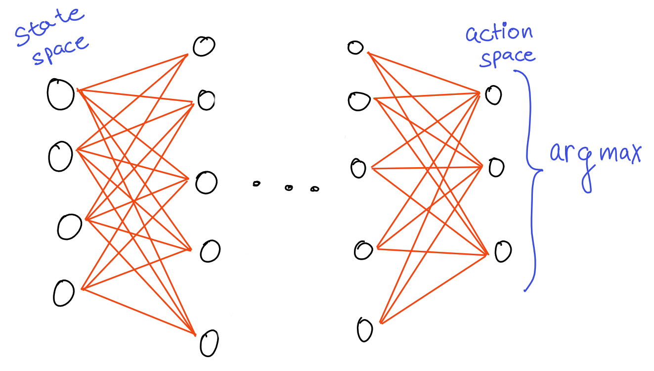
Learning a neural network is essentially the problem of finding weights for the net which maximize (or minimize) some objective function, like the score obtained. Traditionally, this optimization is done using gradient descent (or related algorithms) - if our objective function is differentiable wrt to the parameters, and perhaps more importantly, the gradient is easy to compute, we update the parameters by travelling along the gradient(either ascending or descending, depending on if we want to maximize or minimize).
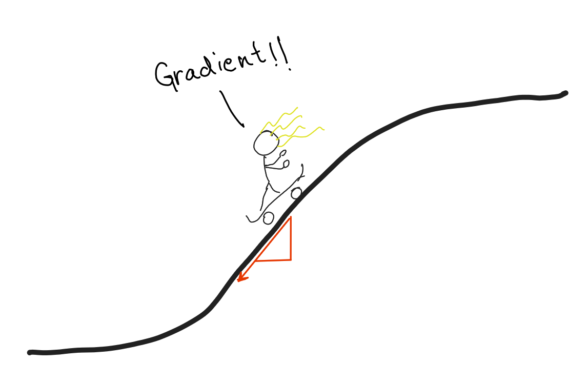
Most gradient based algorithms rely on approximating the reward as some differentiable function, for which computing the gradient is feasible.
Gradient Evolution, but why?
Evolutionary algorithms are another class of optimization algorithms that can be used for training neural networks, which mimic natural selection and genetic mutation and attempt to find optimal parameters for our NN function. Some famous evolutionary algorithms include NEAT, E-GAN etc.
A natural question to ask is - can we do better than random mutations? Randomly mutating provides one way of exploring the search space, but it is similar to flailing in the dark, hoping to hit a light switch. We might try to think of a hybrid algorithm between gradient based and purely random evolutionary algorithms. One such algorithm is Gradient Evolution.
Consider a reward function \(f : \mathbb{R}^n \to \mathbb{R}\) (for example, in the case of AI playing a game, \(f\) is the score obtained by the AI (neural network) playing the game). We have access to the function as a black-box; internally the function might be extremely complex. The simplest evolutionary algorithm that we might use is to take a population \({\theta_1, \theta_2, \cdots \theta_{n}}, \theta_i \in \mathbb{R}^n\), randomly mutate a few top samples (those with highest value of \(f\)), and, out of all the samples, pick the \(n\) best samples as our next generation. In successive generations, we expect to get better and better scores; however, this has no guarantees.
Instead of random mutations, we may use the gradient to guarantee increase in our scores; however, computing the gradient becomes difficult if we have no clue about \(f\).
Gradient Evolution, but how?
The main idea behind gradient evolution is to approximate the gradient using only function calls to \(f\).
The directional derivative of \(f\) at some point \(\theta\), along a direction \(\eta\), is given by \[ \nabla_\eta f(\theta) = \lim_{t \to 0} \frac{f(\theta+t\eta) - f(\theta)}{t} \] One important observation is that the directional derivative can be approximated using function calls as a finite difference: \[ \nabla_\eta f(\theta) \approx \frac{f(\theta+t\eta) - f(\theta)}{t}, \ 0 < t < 1 \]
The gradient has the special property (indeed, this can be viewed as the defining property) that it is the unique vector \(\nabla f(\theta)\) such that, for all directions \(\eta\), the directional derivative along \(\eta\) is equal to the dot product of \(\eta\) and the gradient: \[ \eta \cdot \nabla f(\theta) = \nabla_\eta f(\theta) \]
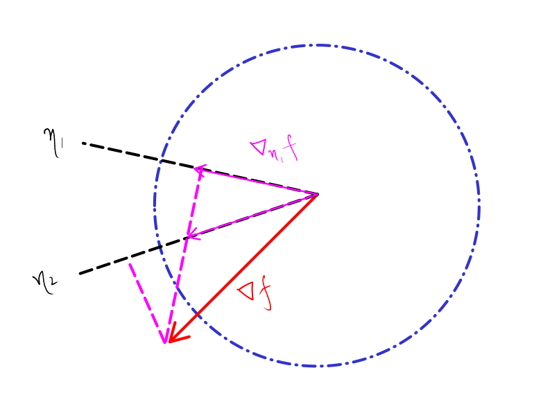
Therefore, if we know the directional derivative along some vector, we know the component of the gradient along that direction. This allows us to reconstruct some part of the gradient. If we knew the component along \(n\) such linearly independent directions, we will be able to reconstruct the gradient precisely; however, this is practically very expensive, as \(n\) can be very large. So, we compute some \(d\) directional derivatives (which, remember, we can do using function calls), and then get an approximation of the gradient.
This approximate gradient can be used in place of the random permutations of the evolutionary algorithm.
The reconstruction problem of the gradient can be written as a linear equation: \(\mathbf{A}x = b\) where the matrix \(\mathbf{A}\) is a \(d \times n\) matrix with the directions \(\eta_1, \eta_2, \cdots, \eta_d\) as the rows, and \(b\) is the vector with the directional derivatives: \(b_i = \nabla_{\eta_i} f(\theta)\). This can be solved using least squares methods. However since we are free to choose the directions as we want, it is best to choose \(d\) orthonormal vectors such as \(d\) random basis vectors. Also, it is best to keep changing these directions in each iteration to get maximum exploration.
Experiments
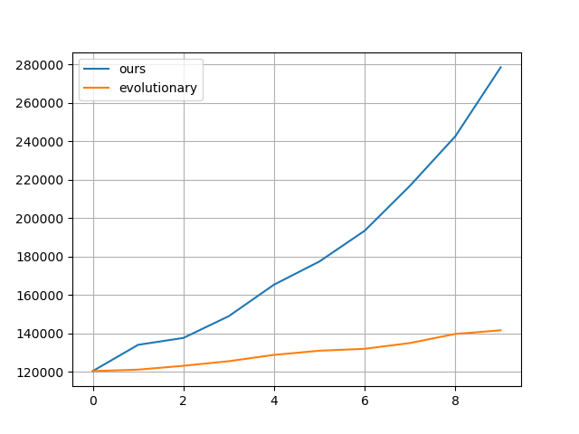
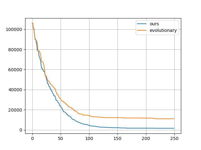
As a proof of concept, consider a standard test function for optimization functions, the Rastrigin Function. We take this as a blackbox and compare the performance against other classical evolutionary algorithms.
| Maximization problem: | Minimization problem: |
|---|---|
 |
 |
Next we considered some OpenAI environments. We tried lander and the Bipedal Walker.
| Gradient evolution: | Normal ES: |
|---|---|
 |
 |
 |
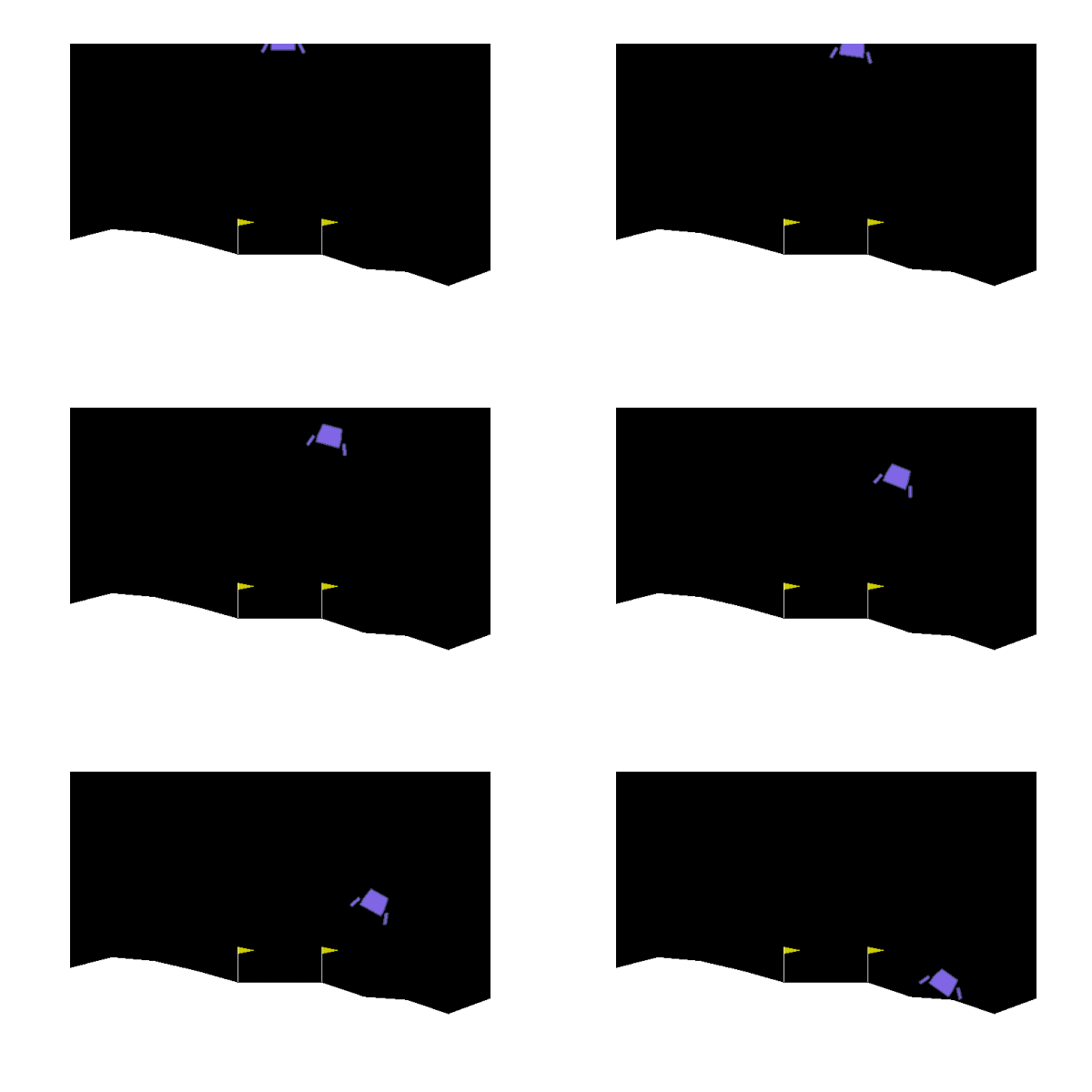 |
The code and results are available here.
Pros and Cons
The major advantage of Gradient Evolution over classical RL techniques is its highly parallizable nature and search space exploration. Since we don’t need any sort of backpropagation, the neural network implementation reduces to a buch of matrix multiplications. unlike other RL algorithms that try to model the value function of the environment, this algorithm treats the reward function as a black box (and therefore falls under the category of blackbox optimization). Moreover, unlike the classical evolutionary algorithms, gradient evolution does not have entirely random mutations.
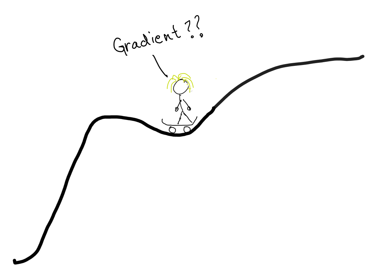
However, the algorithm also has a few major drawbacks. As with any gradient-based algorithm, the evolution might get stuck in local optimums, where the gradient becomes very small. There are a few ways to get around this problem, but it nevertheless remains a nuisance. Also, many functions might actually be very ill-behaved where gradient might not give a very good idea for how to explore. For example, the function might consist of largely flat terrain, with little curvature, and large values only at certain points. In such a case, computing gradients would not be very worthwhile, and simple evolutionary strategies might be better.
Final Thoughts
For further reading on gradient evolution, we suggest the this paper. For a better reading on nature inspired algorithms in general, we suggest Nature-Inspired Algorithms for Optimisation by Thomas Weise, Michael Zapf, Raymond Chiong, Antonio J. Nebro(the gradient evolution algorithm is explained in the chapter The Evolutionary-Gradient-Search Procedure in Theory and Practice).
Gradient evolution is an example of a broader class of algorithms inspired by nature called Evolutionary and Genetic Algorithms. We have barely scratched the surface of this vast field. We may talk more about such algorithms in future posts.
Apart from evolutionary algorithms, another class of algorithms for predictive control with huge applicability is the class of Reinforcement Learning (RL) algorithms. We may also take more about them in the future.
For any issues, suggestions, or questions, reach out to us at roomnumber308@gmail.com.